Practice AHL 4.13—Non-linear regression with authentic IB Mathematics Applications & Interpretation (AI) exam questions for both SL and HL students. This question bank mirrors Paper 1, 2, 3 structure, covering key topics like core principles, advanced applications, and practical problem-solving. Get instant solutions, detailed explanations, and build exam confidence with questions in the style of IB examiners.
Elena is modeling the decay of a radioactive substance. The mass, (in grams), remaining after days is given by:
| 0 | 5 | 10 | 15 | |
|---|---|---|---|---|
| 100 | 60.7 | 36.8 | 22.3 |
She proposes a model of the form , where and are positive constants.
Show that the model satisfies the differential equation .
Find the values of and using a logarithmic transformation and least squares regression.
Estimate the mass remaining after 20 days.
Calculate the sum of squared residuals for the model at the given data points.
An engineer models the vibration amplitude, (in mm), of a machine as a function of its operating frequency, (in Hz). The data suggests a polynomial relationship:
| 10 | 20 | 30 | 40 | |
|---|---|---|---|---|
| 2.5 | 5.0 | 6.0 | 5.5 |
The engineer proposes a cubic model of the form , where , and are constants.
Find the equation of the least squares cubic regression curve.
Write down the coefficient of determination, , for this model.
Find the frequency at which the amplitude is maximized, using the cubic model.
Calculate the sum of squared residuals for the model at the given points.
Suggest one reason why a cubic model might not be appropriate for frequencies far beyond 40 Hz .
A physicist investigates the cooling of a metal rod after being removed from a furnace. The temperature, (in ), of the rod at time (in minutes) is recorded as:
| 0 | 5 | 10 | 15 | |
|---|---|---|---|---|
| 200 | 150 | 120 | 100 |
The physicist proposes a modified exponential model of the form , where , and are constants, and represents the ambient temperature (assumed to be ).
Show that follows an exponential decay model.
Find the values of and using least squares regression, given .
Calculate the sum of squared residuals for the model.
Predict the temperature after 20 minutes.
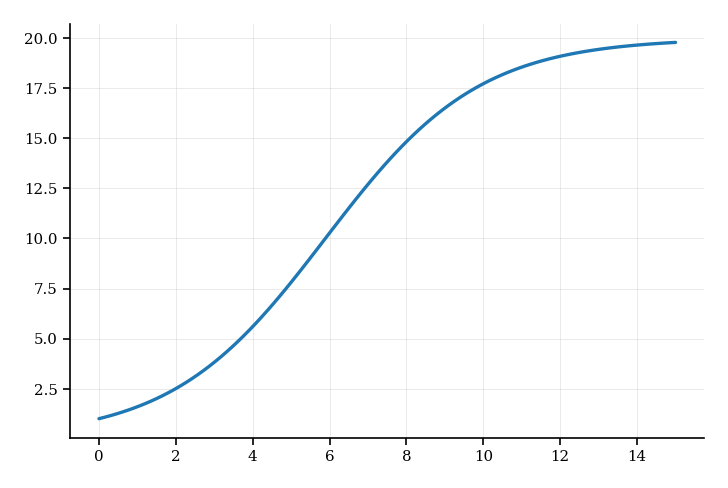
A biologist is studying the growth of a bacterial colony. The number of bacteria, (in thousands), after hours is recorded as follows:
| 0 | 2 | 4 | 6 | |
|---|---|---|---|---|
| 1.0 | 2.5 | 5.6 | 10.3 |
The biologist models the growth using a logistic function of the form , where , and are positive constants. Based on preliminary observations, the carrying capacity is estimated to be 20 thousand.

Explain why a logistic model is appropriate for this data.
[1 mark]
Transform the logistic model into a linear form to estimate parameters using regression.
[2 marks]
Using and the linear form from Part 2, estimate the values of and using the data provided.
[3 marks]
Predict the number of bacteria after 8 hours.
[2 marks]
Discuss one limitation of using this logistic model for long-term predictions.
[1 mark]
A researcher is studying the relationship between the number of hours spent studying, , and the scores obtained in a test, . The data collected is as follows: .
Using the data provided, find the quadratic regression equation of the curve of best fit.
Using the quadratic regression equation found in part 1, predict the test score for a student who studies for 6 hours.
A researcher is studying the relationship between the amount of fertilizer used (in kg) and the yield of a particular crop (in tons). The data collected is as follows: (2.3, 4.5), (3.1, 5.2), (4.7, 6.8), (5.5, 7.1), (6.2, 8.0), (7.4, 9.3). The researcher believes that a non-linear model would best describe the relationship between these variables.
Using the data provided, fit an exponential regression model of the form to the data. Determine the values of and .
Calculate the coefficient of determination () for the exponential regression model.
Describe what this means about the fit of the model.
A marine biologist models the oxygen concentration, (in ), in a coral reef as a function of time, (in hours), over a 24-hour period. The data suggests a sinusoidal pattern:
| (hours) | 0 | 6 | 12 | 18 | 24 |
|---|---|---|---|---|---|
| () | 6.0 | 7.5 | 6.0 | 4.5 | 6.0 |
The biologist proposes a model of the form , where , and are constants.
Show that the period of the proposed model is .
Given the data suggests a 24-hour period, find the value of .
Find the values of and using least squares regression.
Calculate the sum of squared residuals for the model at the given points.
Discuss one limitation of this model for predicting oxygen levels beyond 24 hours.
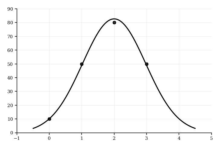
An ecologist models the population density of a species, (in individuals per ), as a function of distance, (in km), from a pollution source. The data suggests a Gaussian distribution:
| 0 | 1 | 2 | 3 | |
|---|---|---|---|---|
| 10 | 50 | 80 | 50 |
The ecologist proposes a model of the form , where , and are constants.

Transform the model into a linear form for regression.
Estimate , and using least squares regression.
Calculate the coefficient of determination, , for the model.
Predict the population density at .
Discuss one limitation of this model for predicting density at large distances.
A research team is evaluating two models to estimate the growth of a bacterial culture over time in hours.
Model X is defined by the linear equation .
Determine the value of the coefficient of determination, , for Model X.
State the equation for Model X.
Use Model X to predict the growth at hours.
A researcher studies the intensity of light, (in lumens), emitted by a bioluminescent organism as a function of time, (in hours), after exposure to a stimulus. The data is recorded as follows:
| (hours) | 0 | 1 | 2 | 3 |
|---|---|---|---|---|
| (lumens) | 50.0 | 41.2 | 35.0 | 30.6 |
The researcher proposes a model of the form , where , and are positive constants, and represents the baseline intensity.
Show that follows an exponential decay model.
Given , find the values of and using least squares regression on the transformed data .
Calculate the sum of squared residuals (SSR) for the model with respect to the given data.
Estimate the light intensity after 4 hours using the model found in part 2.