- IB
- Question Type 3: Finding the quartiles using the cumulative frequency graph
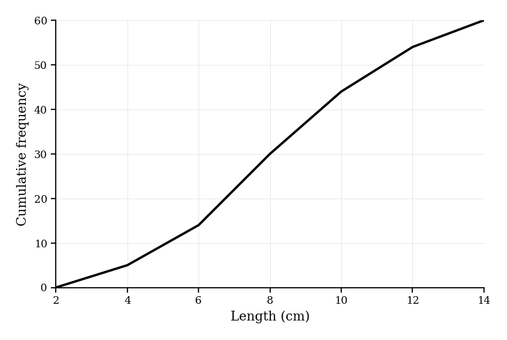
Leaf lengths (cm) for 60 leaves were grouped and a cumulative frequency curve was drawn through the points below.
Data (points on the cumulative frequency curve):
| Upper length (cm) | Cumulative frequency |
|---|---|
| 4 | 5 |
| 6 | 14 |
| 8 | 30 |
| 10 | 44 |
| 12 | 54 |
| 14 | 60 |
![Cumulative frequency graph: x-axis \text{length (cm)} from 2 to 14, y-axis \text{cum. freq.} 0 to 60. Points at (4,5), (6,14), (8,30), (10,44), (12,54), (14,60), joined linearly.]
Estimate the interquartile range (IQR). Give answers to 1 decimal place.
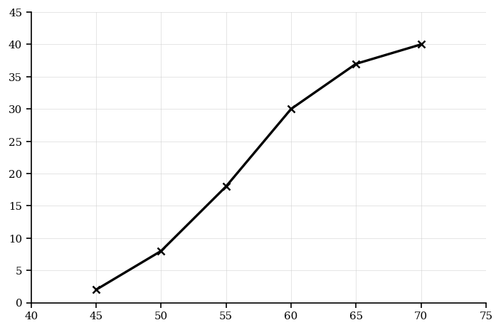
A cumulative frequency graph for 40 adults’ weights (kg) is drawn through the points below.
Data (points on the cumulative frequency curve):
| Upper weight (kg) | Cumulative frequency |
|---|---|
| 45 | 2 |
| 50 | 8 |
| 55 | 18 |
| 60 | 30 |
| 65 | 37 |
| 70 | 40 |
![Cumulative frequency graph: x-axis \text{weight (kg)} 40 to 70, y-axis \text{cum. freq.} 0 to 40, points at (45,2), (50,8), (55,18), (60,30), (65,37), (70,40) joined linearly.]
Estimate , , and the IQR. Give answers to 1 decimal place if needed.
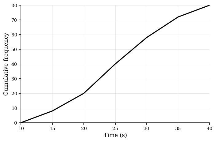
The cumulative frequency graph for 80 athletes’ sprint times (in seconds) is drawn through the points below.
Data (points on the cumulative frequency curve):
| Upper time | Cumulative frequency |
|---|---|
| 15 | 8 |
| 20 | 20 |
| 25 | 40 |
| 30 | 58 |
| 35 | 72 |
| 40 | 80 |
![Cumulative frequency graph: x-axis labelled \text{time (s)} from 10 to 40, y-axis labelled \text{cum. freq.} from 0 to 80. Points at (15,8), (20,20), (25,40), (30,58), (35,72), (40,80), joined linearly.]
Estimate the median and the interquartile range (IQR). Give answers to 1 decimal place where necessary.
Heights (cm) of 48 seedlings are displayed with a cumulative frequency curve through the points below.
Data (points on the cumulative frequency curve):
| Upper height (cm) | Cumulative frequency |
|---|---|
| 54 | 4 |
| 58 | 12 |
| 62 | 24 |
| 66 | 34 |
| 70 | 42 |
| 74 | 48 |
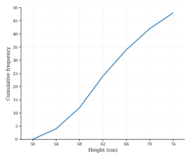
![Cumulative frequency graph: x-axis \text{height (cm)} 50 to 74, y-axis \text{cum. freq.} 0 to 48, points at (54,4), (58,12), (62,24), (66,34), (70,42), (74,48) joined linearly.]
Estimate , median, , and the IQR. Give answers to 1 decimal place where necessary.
The cumulative frequency graph of test scores (out of 60) is drawn by plotting the points below and joining them with straight segments.
Data (points on the cumulative frequency curve):
| Upper score | Cumulative frequency |
|---|---|
| 10 | 4 |
| 20 | 10 |
| 30 | 20 |
| 40 | 32 |
| 50 | 42 |
| 60 | 50 |
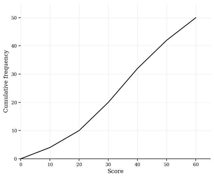
![Cumulative frequency graph: x-axis labelled \text{score} from 0 to 60, y-axis labelled \text{cumulative frequency} from 0 to 50. Points plotted at (10,4), (20,10), (30,20), (40,32), (50,42), (60,50) and joined linearly.]
Estimate , the median, , and the interquartile range (IQR). Give answers to 1 decimal place where necessary.
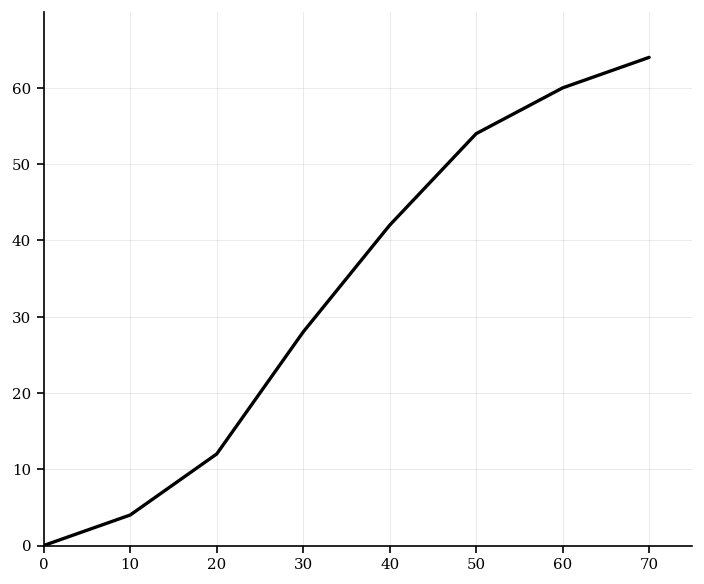
The cumulative frequency graph for ages (years) of 64 museum visitors passes through the points below.
Data (points on the cumulative frequency curve):
| Upper age (years) | Cumulative frequency |
|---|---|
| 10 | 4 |
| 20 | 12 |
| 30 | 28 |
| 40 | 42 |
| 50 | 54 |
| 60 | 60 |
| 70 | 64 |
![Cumulative frequency graph: x-axis \text{age (years)} 0 to 70, y-axis \text{cum. freq.} 0 to 64, points at (10,4), (20,12), (30,28), (40,42), (50,54), (60,60), (70,64) joined linearly.]
Estimate the median and IQR. Give answers to 1 decimal place where necessary.
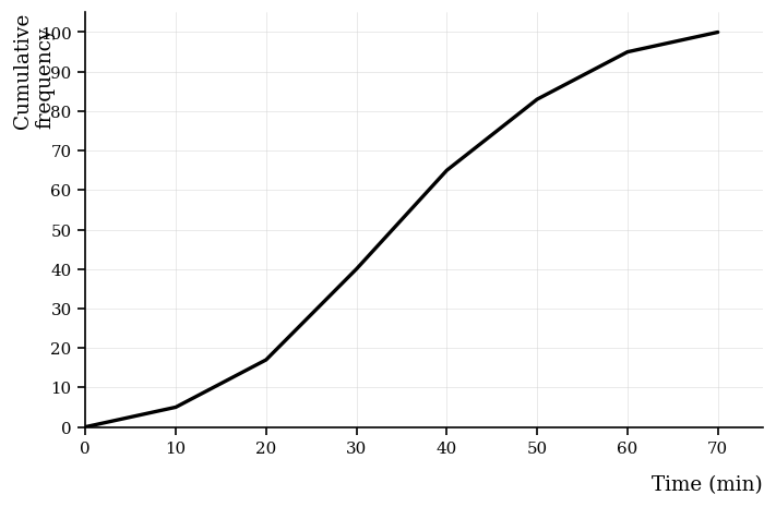
The cumulative frequency graph for 100 commuters’ travel times (minutes) passes through the points below.
Data (points on the cumulative frequency curve):
| Upper time (min) | Cumulative frequency |
|---|---|
| 10 | 5 |
| 20 | 17 |
| 30 | 40 |
| 40 | 65 |
| 50 | 83 |
| 60 | 95 |
| 70 | 100 |
![Cumulative frequency graph: x-axis \text{time (min)} 0 to 70, y-axis \text{cum. freq.} 0 to 100, points at (10,5), (20,17), (30,40), (40,65), (50,83), (60,95), (70,100) joined linearly.]
Estimate the median and IQR. Give answers to 1 decimal place.
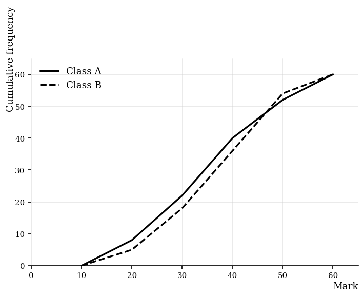
Two classes sat the same test. Their cumulative frequency graphs are summarised by the points below.
Class A data (points on the cumulative frequency curve):
| Upper mark | Cumulative frequency |
|---|---|
| 20 | 8 |
| 30 | 22 |
| 40 | 40 |
| 50 | 52 |
| 60 | 60 |
Class B data (points on the cumulative frequency curve):
| Upper mark | Cumulative frequency |
|---|---|
| 20 | 5 |
| 30 | 18 |
| 40 | 36 |
| 50 | 54 |
| 60 | 60 |
![Two cumulative frequency graphs on the same axes: x-axis \text{mark} 0 to 60, y-axis \text{cum. freq.} 0 to 60. Class A points at (20,8), (30,22), (40,40), (50,52), (60,60). Class B points at (20,5), (30,18), (40,36), (50,54), (60,60). Each set joined linearly.]
For each class, estimate the IQR, then state which class has the larger IQR. Give answers to 1 decimal place where necessary.
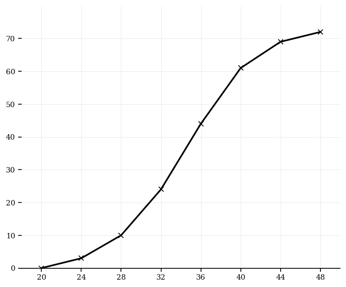
The cumulative frequency graph for metal rod lengths (cm) passes through the points below.
Data (points on the cumulative frequency curve):
| Upper length (cm) | Cumulative frequency |
|---|---|
| 24 | 3 |
| 28 | 10 |
| 32 | 24 |
| 36 | 44 |
| 40 | 61 |
| 44 | 69 |
| 48 | 72 |
![Cumulative frequency graph: x-axis \text{length (cm)} 20 to 48, y-axis \text{cum. freq.} 0 to 72, points at (24,3), (28,10), (32,24), (36,44), (40,61), (44,69), (48,72) joined linearly.]
Estimate , the median, , and the IQR. Give answers to 1 decimal place where necessary.
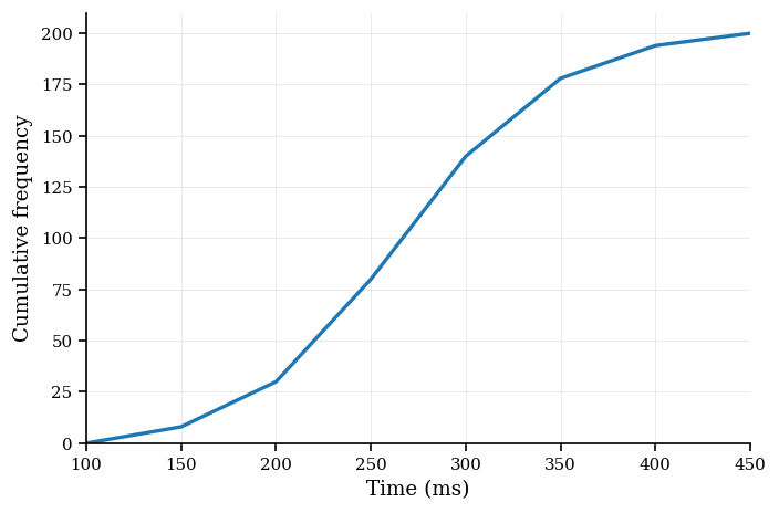
Reaction times (ms) for 200 participants are summarized by the cumulative frequency curve through the points below.
Data (points on the cumulative frequency curve):
| Upper time (ms) | Cumulative frequency |
|---|---|
| 150 | 8 |
| 200 | 30 |
| 250 | 80 |
| 300 | 140 |
| 350 | 178 |
| 400 | 194 |
| 450 | 200 |
![Cumulative frequency graph: x-axis \text{time (ms)} 100 to 450, y-axis \text{cum. freq.} 0 to 200, points at (150,8), (200,30), (250,80), (300,140), (350,178), (400,194), (450,200) joined linearly.]
Estimate the median and the IQR. Give answers to 1 decimal place where necessary.
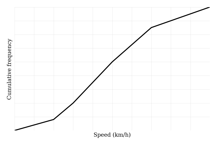
The cumulative frequency graph for car speeds (km/h) is based on unequal class widths and passes through the points below.
Data (points on the cumulative frequency curve):
| Upper speed (km/h) | Cumulative frequency |
|---|---|
| 120 | 8 |
| 130 | 20 |
| 150 | 50 |
| 170 | 75 |
| 200 | 90 |
![Cumulative frequency graph: x-axis \text{speed (km/h)} 100 to 200, y-axis \text{cum. freq.} 0 to 90, points at (120,8), (130,20), (150,50), (170,75), (200,90), joined linearly despite unequal widths.]
Estimate , the median, , and the IQR. Give answers to 1 decimal place where necessary.
A cumulative frequency graph for 50 task completion times (minutes) includes a zero-frequency class. The curve passes through the points below.
Data (points on the cumulative frequency curve):
| Upper time (min) | Cumulative frequency |
|---|---|
| 5 | 6 |
| 10 | 20 |
| 12 | 20 |
| 20 | 40 |
| 30 | 50 |
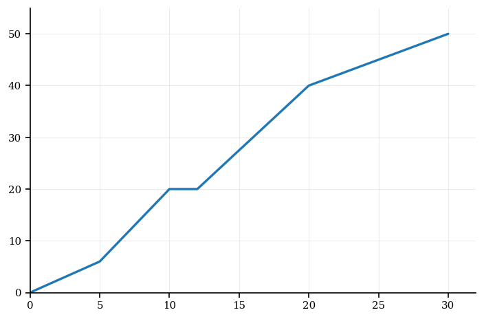
![Cumulative frequency graph: x-axis \text{time (min)} 0 to 30, y-axis \text{cum. freq.} 0 to 50. Points at (5,6), (10,20), (12,20) showing a plateau, then (20,40), (30,50), joined linearly.]
Estimate the median and the IQR. Give answers to 1 decimal place where necessary.